Tutorial

We first load necessary packages.

using CairoMakie
using Fermions
using LinearAlgebra
using RAS_DMFT

Non-interacting Bethe lattice in infinite dimensions

The non-interacting density is the Wigner semicircle distribution

\[ρ(ω) = \frac{2}{πD^2}\sqrt{D^2 - ω^2}\]

from which we can define a non-interacting Green's function $G(ω)$ with the relation

\[ρ(ω) = -\frac{1}{π}\mathrm{Im}G(ω).\]

Let us plot it:

D = 1.0 # half-bandwith
W = range(-2 * D, 2 * D; length = 1_000) # frequency grid
g = greens_function_bethe_analytic(W, D)

f = Figure();
ax = Axis(f[1, 1]; xlabel = L"ω/D", ylabel = L"DG")
lines!(ax, W, real(g); label = L"\mathrm{Re}~G_0")
lines!(ax, W, imag(g); label = L"\mathrm{Im}~G_0")
axislegend(ax; position = :lt)
xlims!(ax, first(W), last(W))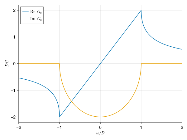

For calculations, we need to discretize this to $n_\mathrm{bath}$ points:

n_bath = 51 # number of bath sites
grid = range(-D, D; length = n_bath) # linear grid (others are possible)
G0 = greens_function_bethe_grid(grid)

PolesSum{Float64, Float64} with 51 poles

This returns a PolesSum instance which only stores locations $ϵ_i$ and weights $w_i$.

f = Figure();
ax = Axis(f[1, 1]; xlabel = "locations", ylabel = "weights")
plot!(ax, locations(G0), weights(G0))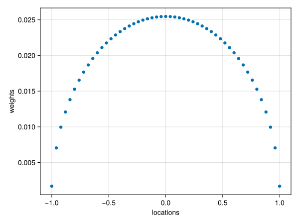

We can see that this looks like a discrete version of our semicircle. Our spectrum is now

\[A(ω) = ∑_i w_i δ(ω - ϵ_i).\]

If we introduce some broadening, this should look like the continuous one. Lorentzian broadening is characterized by $δ$

\[A(ω) = ∑_i w_i \frac{1}{π}\frac{δ}{(ω -ϵ_i)^2 + δ^2},\]

Gaussian one by $σ$

\[A(ω) = ∑_i w_i\frac{1}{\sqrt{2πσ^2}}\exp\left(-\frac{(ω - ϵ_i)^2}{2σ^2}\right).\]

δ = σ = 0.04
f = Figure();
ax = Axis(f[1, 1]; xlabel = L"ω/D", ylabel = L"πDA(ω)")
lines!(ax, W, -imag(g); label = "exact", color = :gray, linewidth = 4)
lines!(ax, W, -imag(evaluate_lorentzian(G0, W, δ)); label = "Lorentzian")
lines!(ax, W, -imag(evaluate_gaussian(G0, W, σ)); label = "Gaussian")
axislegend(ax; position = :lt)
xlims!(ax, first(W), last(W))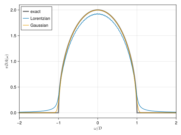

DMFT step

For all following calculations we set our unit of energy to $D=1$.

Impurity

Values for the half-filled impurity. A value of $U/D=2.0$ will generate a strongly correlated metal.

U = 2.0 # Coulomb interaction
μ = U / 2 # chemical potential
ϵ_imp = -μ # energy level for half-filling

-1.0

Restrictions for our active space.

L = 1 # number of chain sites to be treated exactly
p = 2 # order of excitations for remaining chains

2

Operators for exact part. This is necessary to introduce the interacting part and Hartree term. One can also introduce other operators, e.g., $S_z$, $S^2$ and measure their expectation values.

fs = FockSpace(Orbitals(2 + 2 * L), FermionicSpin(1 // 2))
c = annihilators(fs)
n = occupations(fs)
H_int = U * n[1, 1 // 2] * n[1, -1 // 2] # interacting Hamiltonian
d_dag = c[1, -1 // 2]' # d_↓^†
q_dag = H_int * d_dag - d_dag * H_int  # auxiliary operator q_↓^† = [H_int, d^†]
# measure these on ground state
O_Σ_H = q_dag' * d_dag + d_dag * q_dag' # Operator for Hartree term
d_occ = n[1, 1 // 2] * n[1, -1 // 2] # double occupation

Fermions.Operator{Int64, Fermions.FockSpaces.FockSpace{UInt64, UInt64, Tuple{Fermions.FockSpaces.Orbitals, Fermions.FockSpaces.FermionicSpin}}, Vector{Fermions.Terms.Term{Int64, UInt64, UInt64}}} for 8 flavours (1 terms):
1 n[1, -1//2] n[1, 1//2]

Hybridization function

On the Bethe lattice, the hybridization function $Δ$ is nothing more than a rescaled Green's function

\[Δ(ω) = \frac{D^2}{4} G(ω).\]

We can create one using

grid = range(-4 * D, 4 * D; length = n_bath) # linear grid
Δ0 = hybridization_function_bethe_grid(grid)
remove_zero_weight!(Δ0)

PolesSum{Float64, Float64} with 13 poles

Here, we set our grid to $[-4D, 4D]$. This will initially create poles with zero weight. Due to the Coulomb interaction $U$, spectral weight will move to higher frequencies, such that poles with initially no weight will obtain a finite value in successive calculations.

Ground state

We can then calculate the ground state up to a user-given variance of the Hamiltonian $\mathrm{var}(H)$. Next to the bare level $ϵ_\mathrm{imp}$ entering the Hamiltonian, the mean-field level $ϵ_\mathrm{mf}$ selects the natural impurity orbital basis. Both vanish here, because the system is particle-hole symmetric at half filling.

var = 1.0e-10
H, E0, ψ0 = init_system(Δ0, H_int, ϵ_imp, 0, L, L, p, var);

Given our ground state, we can calculate expectation values with LinearAlgebra.dot.

dot(ψ0, d_occ, ψ0) # expectation value
Σ_H = dot(ψ0, O_Σ_H, ψ0) # Hartree term, should be U/2 = 1.0

0.9999999999999991

Block correlator

Shift to create diagonal matrices later.

q_dag_tilde = q_dag - Σ_H * d_dag
O_plus = [q_dag_tilde, d_dag] # for C+
O_minus = map(adjoint, O_plus); # for C-

As we have two operators as input, we will create $2×2$ block correlators. If we use $n$ Krylov steps, each will have $2n$ poles.

n_kryl = 50
C_plus = correlator_plus(H, ψ0, O_plus, n_kryl)
C_minus = correlator_minus(H, ψ0, O_minus, n_kryl)
C = transpose(C_minus) + C_plus

PolesSumBlock{Float64, Float64} with 200 poles of size 2×2

We can plot the spectrum. The Green's function is the $[2,2]$ component.

G = PolesSum(C, 2, 2)
f = Figure();
ax = Axis(f[1, 1]; xlabel = L"ω/D", ylabel = L"πDA(ω)")
lines!(ax, W, -imag(evaluate_gaussian(G, W, σ)))
xlims!(ax, first(W), last(W))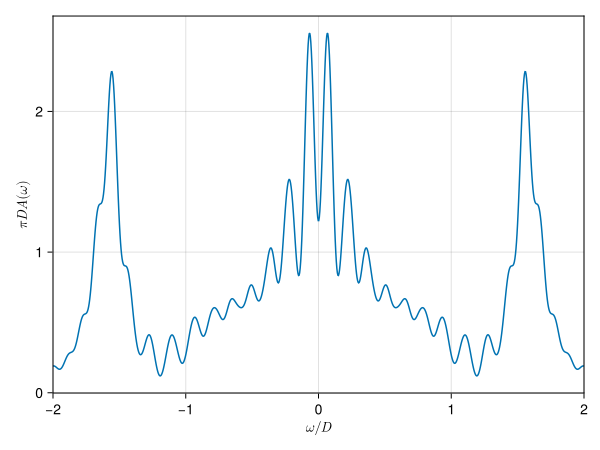

Self-energy

Here, we use the improved symmetric estimator^[Kugler2022], which is evaluated as a Schur complement.

Σ = self_energy_schur(C)
Σ = PolesSum(Σ, 1, 1)
sigma = evaluate_gaussian(Σ, W, σ)
f = Figure();
ax = Axis(f[1, 1]; xlabel = L"ω/D", ylabel = L"Σ(ω)/D")
lines!(ax, W, real(sigma); label = L"\mathrm{Re}~Σ")
lines!(ax, W, imag(sigma); label = L"\mathrm{Im}~Σ")
axislegend(ax; position = :lt)
xlims!(ax, first(W), last(W))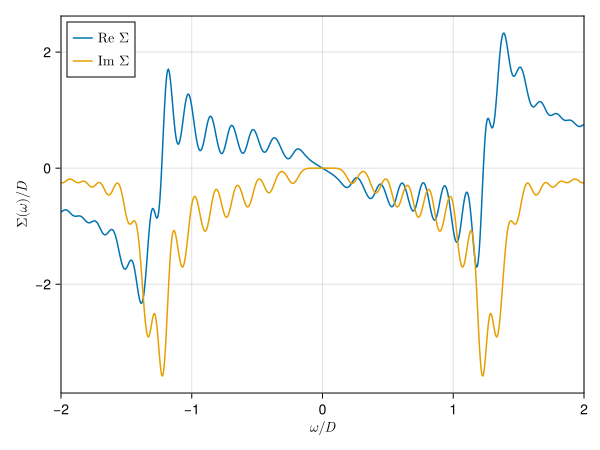

We can calculate the quasiparticle weight

\[\begin{aligned} Z &= \left(1 - \left.\frac{∂\mathrm{Re}~Σ}{∂ω}\right|_{ω=0}\right)^{-1} \\ &= \left(1 + \sum_i \frac{w_i}{ϵ_i^2}\right)^{-1} \end{aligned}\]

directly on the real axis without the use of a difference quotient. Due to poles at $ϵ_i≈0$ this will diverge, and poles with small weight need to be ignored. This is controlled by the second parameter.

quasiparticle_weight(Σ; tol = sqrt(eps()))

0.4353854000821964

Update hybridization

At the end of each DMFT step, we have to update the hybridization function using the new self-energy.

Δ = update_hybridization_function(Δ0, μ, Σ_H, Σ)

PolesSum{Float64, Float64} with 2894 poles

As this function has too many poles to be computationally feasible, we put them onto our initial grid

Δ_grid = to_grid(Δ, grid)

PolesSum{Float64, Float64} with 51 poles

We can then put this as our next input and continue at Ground state.

This page was generated using Literate.jl.